The Fundamental Theorem of Calculus

When we introduced definite integrals, we computed them according to the definition as the limit of Riemann sums and we saw that this procedure is not very easy. In fact, there is a much simpler method for evaluating integrals.

We already discovered it when we talked about the area problem for the first time.

There, we introduced a function ${P}{\left({x}\right)}$ whose value is the area under the function ${f{}}$ on the interval ${\left[{a},{x}\right]}$ ( ${x}$ can vary from ${a}$ to ${b}$ ).

Now, when we know about definite integrals, we can write that ${P}{\left({x}\right)}={\int_{{a}}^{{x}}}{f{{\left({t}\right)}}}{d}{t}$ (note that we changed $x$ to $t$ under the integral in order not to mix it with the upper limit).

Also, we discovered the Newton-Leibniz formula, which states that ${P}'{\left({x}\right)}={f{{\left({x}\right)}}}$ and ${P}{\left({x}\right)}={F}{\left({x}\right)}-{F}{\left({a}\right)}$ , where ${F}'={f{}}$ .

Here, we are going to formalize this result and give another proof, because these facts are very important in calculus: they connect differential calculus with integral calculus.

Fundamental Theorem of Calculus. Suppose that ${f{}}$ is continuous on ${\left[{a},{b}\right]}$ .

If ${P}{\left({x}\right)}={\int_{{a}}^{{x}}}{f{{\left({t}\right)}}}{d}{t}$ , then ${P}'{\left({x}\right)}={f{{\left({x}\right)}}}$ .
${\int_{{a}}^{{b}}}{f{{\left({x}\right)}}}{d}{x}={F}{\left({b}\right)}-{F}{\left({a}\right)}$ , where F is any antiderivative of ${f{}}$ , that is ${F}'={f{}}$ .

Part 1 can be rewritten as $\frac{{d}}{{{d}{x}}}{\int_{{a}}^{{x}}}{f{{\left({t}\right)}}}{d}{t}={f{{\left({x}\right)}}}$ , which says that if ${f{}}$ is integrated and then the result is differentiated, we arrive back at the original function.

Part 2 can be rewritten as ${\int_{{a}}^{{b}}}{F}'{\left({x}\right)}{d}{x}={F}{\left({b}\right)}-{F}{\left({a}\right)}$ , and it says that if we take a function ${F}$ , first differentiate it, and then integrate the result, we arrive back at the original function ${F}$ but in the form ${F}{\left({b}\right)}-{F}{\left({a}\right)}$ .

The fundamental theorem of calculus says that differentiation and integration are the inverse processes.

Proof of Part 1. Let ${P}{\left({x}\right)}={\int_{{a}}^{{x}}}{f{{\left({t}\right)}}}{d}{t}$ . If ${x}$ and ${x}+{h}$ are in the open interval ${\left({a},{b}\right)}$ , then ${P}{\left({x}+{h}\right)}-{P}{\left({x}\right)}={\int_{{a}}^{{{x}+{h}}}}{f{{\left({t}\right)}}}{d}{t}-{\int_{{a}}^{{x}}}{f{{\left({t}\right)}}}{d}{t}$ .

Now, use the adjacency property of the integral: ${\int_{{a}}^{{{x}+{h}}}}{f{{\left({t}\right)}}}{d}{t}-{\int_{{a}}^{{x}}}{f{{\left({t}\right)}}}{d}{t}={\left({\int_{{a}}^{{x}}}{f{{\left({t}\right)}}}{d}{t}+{\int_{{x}}^{{{x}+{h}}}}{f{{\left({t}\right)}}}{d}{t}\right)}-{\int_{{a}}^{{x}}}{f{{\left({t}\right)}}}{d}{t}={\int_{{x}}^{{{x}+{h}}}}{f{{\left({t}\right)}}}{d}{t}$ .

Now, apply the mean value theorem for integrals:

${\int_{{x}}^{{{x}+{h}}}}{f{{\left({t}\right)}}}{d}{t}={n}{\left({x}+{h}-{x}\right)}={n}{h}$ , where ${m}'\le{n}\le{M}'$ ( ${M}'$ is the maximum value, and ${m}'$ is the minimum value of ${f{}}$ on ${\left[{x},{x}+{h}\right]}$ ).

So, we obtained that ${P}{\left({x}+{h}\right)}-{P}{\left({x}\right)}={n}{h}$ . If we let ${h}\to{0}$ , then ${P}{\left({x}+{h}\right)}-{P}{\left({x}\right)}\to{0}$ , or ${P}{\left({x}+{h}\right)}\to{P}{\left({x}\right)}$ .

This proves that ${P}{\left({x}\right)}$ is a continuous function.

Without the loss of generality, assume that ${h}>{0}$ .

Since ${f{}}$ is continuous on ${\left[{x},{x}+{h}\right]}$ , the extreme value theorem says that there are numbers ${c}$ and ${d}$ in ${\left[{x},{x}+{h}\right]}$ such that ${f{{\left({c}\right)}}}={m}$ and ${f{{\left({d}\right)}}}={M}$ , where ${m}$ and ${M}$ are the minimum and maximum values of ${f{}}$ on ${\left[{x},{x}+{h}\right]}$ .

According to the comparison property, we have ${m}{\left({x}+{h}-{x}\right)}\le{\int_{{x}}^{{{x}+{h}}}}{f{{\left({t}\right)}}}{d}{t}\le{M}{\left({x}+{h}-{h}\right)}$ , or ${m}{h}\le{\int_{{x}}^{{{x}+{h}}}}{f{{\left({t}\right)}}}{d}{t}\le{M}{h}$ .

This can be divided by ${h}>{0}$ : ${m}\le\frac{{1}}{{h}}{\int_{{x}}^{{{x}+{h}}}}{f{{\left({t}\right)}}}{d}{t}\le{M}$ , or ${m}\le\frac{{{P}{\left({x}+{h}\right)}-{P}{\left({x}\right)}}}{{h}}\le{M}$ .

Finally, ${f{{\left({c}\right)}}}\le\frac{{{P}{\left({x}+{h}\right)}-{P}{\left({x}\right)}}}{{h}}\le{f{{\left({d}\right)}}}$ .

This inequality can be proved for ${h}<{0}$ similarly.

Now, we let ${h}\to{0}$ .

Then, ${c}\to{x}$ , and ${d}\to{x}$ , since ${c}$ and ${d}$ lie between ${x}$ and ${x}+{h}$ .

So, $\lim_{{{h}\to{0}}}{f{{\left({c}\right)}}}=\lim_{{{c}\to{x}}}{f{{\left({c}\right)}}}={f{{\left({x}\right)}}}$ , and $\lim_{{{h}\to{0}}}{f{{\left({d}\right)}}}=\lim_{{{d}\to{x}}}{f{{\left({d}\right)}}}={f{{\left({x}\right)}}}$ because ${f{}}$ is continuous.

Therefore, from the last inequality and the squeeze theorem, we conclude that $\lim_{{{h}\to{0}}}\frac{{{P}{\left({x}+{h}\right)}-{P}{\left({x}\right)}}}{{h}}={f{{\left({x}\right)}}}$ .

But we recognize in the left part the derivative of ${P}{\left({x}\right)}$ ; therefore, ${P}'{\left({x}\right)}={f{{\left({x}\right)}}}$ .

Proof of Part 2. We divide the interval ${\left[{a},{b}\right]}$ into ${n}$ subintervals with the endpoints ${x}_{{0}}{\left(={a}\right)},{x}_{{1}},{x}_{{2}},\ldots,{x}_{{n}}{\left(={b}\right)}$ and with the width of a subinterval $\Delta{x}=\frac{{{b}-{a}}}{{n}}$ . Let ${F}$ be any antiderivative of ${f{}}$ . By subtracting and adding the like terms, we can express the total difference in the ${F}$ values as the sum of the differences over the subintervals: ${F}{\left({b}\right)}-{F}{\left({a}\right)}={F}{\left({x}_{{n}}\right)}-{F}{\left({x}_{{0}}\right)}=$

$={F}{\left({x}_{{n}}\right)}-{F}{\left({x}_{{{n}-{1}}}\right)}+{F}{\left({x}_{{{n}-{2}}}\right)}+\ldots+{F}{\left({x}_{{2}}\right)}-{F}{\left({x}_{{1}}\right)}+{F}{\left({x}_{{1}}\right)}-{F}{\left({x}_{{0}}\right)}=$

$={\sum_{{{i}={1}}}^{{n}}}{\left({F}{\left({x}_{{i}}\right)}-{F}{\left({x}_{{{i}-{1}}}\right)}\right)}$ .

Now, ${F}$ is continuous (because it’s differentiable), and so we can apply the mean value theorem to ${F}$ on each subinterval ${\left[{x}_{{{i}-{1}}},{x}_{{i}}\right]}$ .

Thus, there exists a number ${{x}_{{i}}^{{\star}}}$ between ${x}_{{{i}-{1}}}$ and ${x}_{{i}}$ such that ${F}{\left({x}_{{i}}\right)}-{F}{\left({x}_{{{i}-{1}}}\right)}={F}'{\left({{x}_{{i}}^{{\star}}}\right)}{\left({x}_{{i}}-{x}_{{{i}-{1}}}\right)}={f{{\left({{x}_{{i}}^{{\star}}}\right)}}}\Delta{x}$ .

Therefore, ${F}{\left({b}\right)}-{F}{\left({a}\right)}={\sum_{{{i}={1}}}^{{n}}}{f{{\left({{x}_{{i}}^{{\star}}}\right)}}}\Delta{x}$ .

Now, we take the limit of each side of this equation as ${n}\to\infty$ . The left side is a constant and the right side is a Riemann sum for the function ${f{}}$ ; so, ${F}{\left({b}\right)}-{F}{\left({a}\right)}=\lim_{{{n}\to\infty}}{\sum_{{{i}={1}}}^{{n}}}{f{{\left({{x}_{{i}}^{{\star}}}\right)}}}\Delta{x}={\int_{{a}}^{{b}}}{f{{\left({x}\right)}}}{d}{x}$ .

This finishes the proof of the fundamental theorem of calculus.

When using the evaluation theorem, the following notation is used: ${F}{\left({b}\right)}-{F}{\left({a}\right)}={F}{\left({x}\right)}{{\mid}_{{a}}^{{b}}}={{\left[{F}{\left({x}\right)}\right]}_{{a}}^{{b}}}$ .

We've already talked about the introduced function ${P}{\left({x}\right)}={\int_{{a}}^{{x}}}{f{{\left({t}\right)}}}{d}{t}$ .

We're going to talk about it again because it is a new type of function. It is just like any other functions (power or exponential): for any ${x}$ , ${\int_{{a}}^{{x}}}{f{{\left({t}\right)}}}{d}{t}$ gives a definite number. Sometimes we can represent ${P}{\left({x}\right)}$ in terms of the functions we know, sometimes not.

For example, we know that ${\left(\frac{{1}}{{3}}{{x}}^{{3}}\right)}'={{x}}^{{2}}$ ; so, according to the fundamental theorem of calculus, ${P}{\left({x}\right)}={\int_{{0}}^{{x}}}{{t}}^{{2}}{d}{t}=\frac{{1}}{{3}}{{x}}^{{3}}-\frac{{1}}{{3}}\cdot{{0}}^{{3}}=\frac{{1}}{{3}}{{x}}^{{3}}$ . Here, we expressed ${P}{\left({x}\right)}$ in terms of a power function.

But we can't represent it in terms of elementary functions, for example, the function ${P}{\left({x}\right)}={\int_{{0}}^{{x}}}{{e}}^{{{{x}}^{{2}}}}{d}{x}$ , because we don't know what the antiderivative of ${{e}}^{{{{x}}^{{2}}}}$ is. What we can do is just find the value of ${P}{\left({x}\right)}$ for any given ${x}$ .

Geometrically, ${P}{\left({x}\right)}$ can be interpreted as the net area under the graph of ${f{}}$ from ${a}$ to ${x}$ , where ${x}$ can vary from ${a}$ to ${b}$ . (Think of $P$ as an "area so far" function.)

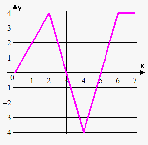
Example 1. The graph of ${f{}}$ is given below. If ${P}{\left({x}\right)}={\int_{{0}}^{{x}}}{f{{\left({t}\right)}}}{d}{t}$ , find ${P}{\left({0}\right)}$ , ${P}{\left({1}\right)}$ , ${P}{\left({2}\right)}$ , ${P}{\left({3}\right)}$ , ${P}{\left({4}\right)}$ , ${P}{\left({6}\right)}$ , and ${P}{\left({7}\right)}$ . Sketch the rough graph of ${P}$ .

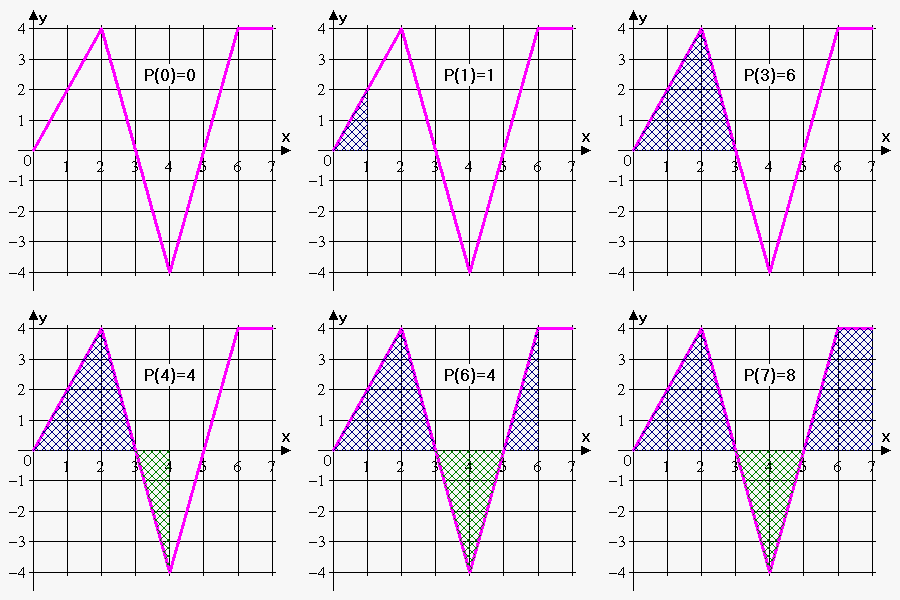
integral as function We immediately have that ${P}{\left({0}\right)}={\int_{{0}}^{{0}}}{f{{\left({t}\right)}}}{d}{t}={0}$ . We can see that ${P}{\left({1}\right)}={\int_{{0}}^{{1}}}{f{{\left({t}\right)}}}{d}{t}$ is the area of the triangle with the sides $1$ and $2$ . Therefore, ${P}{\left({1}\right)}=\frac{{1}}{{2}}\cdot{1}\cdot{2}={1}$ .

We see that ${P}{\left({2}\right)}={\int_{{0}}^{{2}}}{f{{\left({t}\right)}}}{d}{t}$ is the area of the triangle with the sides $2$ and $4$ . So, ${P}{\left({2}\right)}=\frac{{1}}{{2}}\cdot{2}\cdot{4}={4}$ .

The area from $0$ to $3$ consists of the area from $0$ to $2$ and the area from $2$ to $3$ (the triangle with the sides $1$ and $4$ ):

${P}{\left({3}\right)}={\int_{{0}}^{{3}}}{f{{\left({t}\right)}}}{d}{t}={\int_{{0}}^{{2}}}{f{{\left({t}\right)}}}{d}{t}+{\int_{{2}}^{{3}}}{f{{\left({t}\right)}}}{d}{t}={4}+\frac{{1}}{{2}}\cdot{1}\cdot{4}={6}$ .

Similarly, ${P}{\left({4}\right)}={P}{\left({3}\right)}+{\int_{{3}}^{{4}}}{f{{\left({t}\right)}}}{d}{t}$ . But the area of the triangle on interval ${\left[{3},{4}\right]}$ lies below the x-axis, so we subtract it: ${P}{\left({4}\right)}={6}-\frac{{1}}{{2}}\cdot{1}\cdot{4}={4}$ . example of integral as function

Now, ${P}{\left({5}\right)}={P}{\left({4}\right)}+{\int_{{4}}^{{5}}}{f{{\left({t}\right)}}}{d}{t}={4}-\frac{{1}}{{2}}\cdot{1}\cdot{4}={2}$ .

${P}{\left({6}\right)}={P}{\left({5}\right)}+{\int_{{5}}^{{6}}}{f{{\left({t}\right)}}}{d}{t}={2}+\frac{{1}}{{2}}\cdot{1}\cdot{4}={4}$ .

Finally, ${P}{\left({7}\right)}={P}{\left({6}\right)}+{\int_{{6}}^{{7}}}{f{{\left({t}\right)}}}{d}{t}$ , where ${\int_{{7}}^{{6}}}{f{{\left({t}\right)}}}{d}{t}$ is the area of the rectangle with the sides $1$ and $4$ . So, ${P}{\left({7}\right)}={4}+{1}\cdot{4}={8}$ .

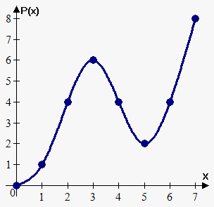
The sketch of ${P}{\left({x}\right)}$ is shown below.

sketch of integral function

Now, we need some more examples for practice.

Example 2. If ${P}{\left({x}\right)}={\int_{{1}}^{{x}}}{{t}}^{{3}}{d}{t}$ , find the formula for ${P}{\left({x}\right)}$ and calculate ${P}'{\left({x}\right)}$ .

Using Part 2 of the fundamental theorem of calculus and the table of indefinite integrals, we have that ${P}{\left({x}\right)}={\int_{{1}}^{{x}}}{{t}}^{{3}}{d}{t}={\left(\frac{{{t}}^{{4}}}{{4}}\right)}{{\mid}_{{1}}^{{x}}}=\frac{{{x}}^{{4}}}{{4}}-\frac{{1}}{{4}}$ .

Now, ${P}'{\left({x}\right)}={\left(\frac{{{x}}^{{4}}}{{4}}-\frac{{1}}{{4}}\right)}'={{x}}^{{3}}$ . We see that ${P}'{\left({x}\right)}={f{{\left({x}\right)}}}$ as expected in accordance with the first part of the fundamental theorem.

Let's work another short example.

Example 3. Find the derivative of ${P}{\left({x}\right)}={\int_{{0}}^{{x}}}\sqrt{{{{t}}^{{3}}+{1}}}{d}{t}$ .

Using the first part of the fundamental theorem of calculus, we have that ${g{'}}{\left({x}\right)}=\sqrt{{{{x}}^{{3}}+{1}}}$ .

Let's move on.

Example 4. Find $\frac{{d}}{{{d}{x}}}{\int_{{2}}^{{{{x}}^{{3}}}}}{\ln{{\left({{t}}^{{2}}+{1}\right)}}}{d}{t}$ .

Here, we have a composite function ${P}{\left({{x}}^{{3}}\right)}$ . To find its derivative, we need to use the chain rule in addition to the fundamental theorem.

Let ${u}={{x}}^{{3}}$ ; then, $\frac{{{d}{u}}}{{{d}{x}}}={\left({{x}}^{{3}}\right)}'={3}{{x}}^{{2}}$ .

$\frac{{d}}{{{d}{x}}}{\int_{{2}}^{{{{x}}^{{3}}}}}{\ln{{\left({{t}}^{{2}}+{1}\right)}}}{d}{t}=\frac{{d}}{{{d}{u}}}{\int_{{2}}^{{u}}}{\ln{{\left({{t}}^{{2}}+{1}\right)}}}\cdot\frac{{{d}{u}}}{{{d}{x}}}=\frac{{d}}{{{d}{u}}}{\int_{{2}}^{{u}}}{\ln{{\left({{t}}^{{2}}+{1}\right)}}}\cdot{3}{{x}}^{{2}}=$

$={\ln{{\left({{u}}^{{2}}+{1}\right)}}}\cdot{3}{{x}}^{{2}}={\ln{{\left({{\left({{x}}^{{3}}\right)}}^{{2}}+{1}\right)}}}\cdot{3}{{x}}^{{2}}={3}{{x}}^{{2}}{\ln{{\left({{x}}^{{6}}+{1}\right)}}}$ .

Now, a couple examples concerning Part 2 of the fundamental theorem.

Example 5. Calculate ${\int_{{0}}^{{5}}}{{e}}^{{x}}{d}{x}$ .

Using Part 2 of the fundamental theorem of calculus and the table of indefinite integrals, we have that ${\int_{{0}}^{{5}}}{{e}}^{{x}}{d}{x}={{e}}^{{x}}{{\mid}_{{0}}^{{5}}}={{e}}^{{5}}-{{e}}^{{0}}={{e}}^{{5}}-{1}$ .

This should be becoming much clearer as we go.

Example 6. Calculate ${\int_{{0}}^{{\frac{\pi}{{2}}}}}{\cos{{\left({x}\right)}}}{d}{x}$ .

Using Part 2 of the fundamental theorem of calculus and the table of indefinite integrals (the antiderivative of ${\cos{{\left({x}\right)}}}$ is ${\sin{{\left({x}\right)}}}$ ), we have that ${\int_{{0}}^{{\frac{\pi}{{2}}}}}{\cos{{\left({x}\right)}}}{d}{x}={\sin{{\left({x}\right)}}}{{\mid}_{{0}}^{{\frac{\pi}{{2}}}}}={\sin{{\left(\frac{\pi}{{2}}\right)}}}-{\sin{{\left({0}\right)}}}={1}$ .

While these examples might seem easy, they are in fact important to memorize what we learned.

Example 7. Find ${\int_{{0}}^{{2}}}{\left({3}{{x}}^{{2}}-{7}\right)}{d}{x}$ .

Using the properties of the definite integral, we can write that ${\int_{{0}}^{{2}}}{\left({3}{{x}}^{{2}}-{7}\right)}{d}{x}={\int_{{0}}^{{2}}}{3}{{x}}^{{2}}{d}{x}-{\int_{{0}}^{{2}}}{7}{d}{x}={3}{\int_{{0}}^{{2}}}{{x}}^{{2}}{d}{x}-{7}{\int_{{0}}^{{2}}}{7}{d}{x}=$

$={3}{\left(\frac{{{x}}^{{3}}}{{3}}\right)}{{\mid}_{{0}}^{{2}}}-{7}\cdot{\left({2}-{0}\right)}={3}{\left(\frac{{8}}{{3}}-\frac{{0}}{{3}}\right)}-{14}=-{6}$ .

And now, our final example.

Example 8. Find ${\int_{{1}}^{{3}}}{\left(\frac{{{2}{{t}}^{{5}}-{8}\sqrt{{{t}}}}}{{t}}+\frac{{7}}{{{{t}}^{{2}}+{1}}}\right)}{d}{t}$ .

First, rewrite the integral a bit: ${\int_{{1}}^{{3}}}{\left(\frac{{{2}{{t}}^{{5}}-{8}\sqrt{{{t}}}}}{{t}}+\frac{{7}}{{{{t}}^{{2}}+{1}}}\right)}{d}{t}={\int_{{1}}^{{3}}}{\left({2}{{t}}^{{4}}-{8}{{t}}^{{-\frac{{1}}{{2}}}}+\frac{{7}}{{{{t}}^{{2}}+{1}}}\right)}{d}{t}$ .

So, ${\int_{{1}}^{{3}}}{\left({2}{{t}}^{{4}}-{8}{{t}}^{{-\frac{{1}}{{2}}}}+\frac{{7}}{{{{t}}^{{2}}+{1}}}\right)}{d}{t}={\left(\frac{{2}}{{5}}{{t}}^{{5}}-{16}\sqrt{{{t}}}+{7}{{\tan}}^{{-{1}}}{\left({t}\right)}\right)}{{\mid}_{{1}}^{{3}}}=$

$={\left(\frac{{2}}{{5}}{{\left({3}\right)}}^{{5}}-{16}\sqrt{{{3}}}+{7}{{\tan}}^{{-{1}}}{\left({3}\right)}\right)}-{\left(\frac{{2}}{{5}}{{\left({1}\right)}}^{{5}}-{16}\sqrt{{{1}}}+{7}{{\tan}}^{{-{1}}}{\left({1}\right)}\right)}=$

$=\frac{{564}}{{5}}-{16}\sqrt{{{3}}}-\frac{{{7}\pi}}{{4}}+{7}{{\tan}}^{{-{1}}}{\left({3}\right)}\approx{88.3327}$ .