Area between Curves
Now, when we know what definite integral is, we can calculate area between curves.
Consider the region $$${S}$$$ that lies between two curves $$${y}={f{{\left({x}\right)}}}$$$ and $$${y}={g{{\left({x}\right)}}}$$$ and between the vertical lines $$${x}={a}$$$ and $$${x}={b}$$$, where $$${f{}}$$$ and $$${g{}}$$$ are continuous functions and $$${f{{\left({x}\right)}}}\ge{g{{\left({x}\right)}}}$$$ for all $$${x}$$$ in $$${\left[{a},{b}\right]}$$$.
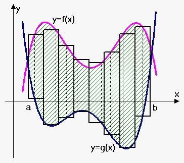 We will proceed in the same fashion as we did when talked about area problem.
Divide region into $$${n}$$$ strips of wdith $$$\Delta{x}=\frac{{{b}-{a}}}{{n}}$$$. We approximate i-th strip by rectangle with base $$$\Delta{x}$$$ and height $$${f{{\left({{x}_{{i}}^{{\star}}}\right)}}}-{g{{\left({{x}_{{i}}^{{\star}}}\right)}}}$$$ where $$${{x}_{{i}}^{{\star}}}\in{\left[{x}_{{{i}-{1}}},{x}_{{i}}\right]}$$$. Thus, approximate area is defined by Riemann sum as $$${A}\approx{\sum_{{{i}={1}}}^{{n}}}{\left({f{{\left({{x}_{{i}}^{{\star}}}\right)}}}-{g{{\left({{x}_{{i}}^{{\star}}}\right)}}}\right)}\Delta{x}$$$. As $$${n}$$$ becomes larger, approximation becomes better.
Therefore, we define area A of S as the limiting value of the sum of the areas of these approximating rectangles: $$${A}=\lim_{{{n}\to\infty}}{\sum_{{{i}={1}}}^{{n}}}{\left({f{{\left({{x}_{{i}}^{{\star}}}\right)}}}-{g{{\left({{x}_{{i}}^{{\star}}}\right)}}}\right)}\Delta{x}$$$.
We recognize in limit definite integral of $$${f{-}}{g{}}$$$.
Formula for Area between Curves. The area $$${A}$$$ of the region bounded by the curves $$${y}={f{{\left({x}\right)}}}$$$ and $$${y}={g{{\left({x}\right)}}}$$$, and the lines $$${x}={a}$$$, $$${x}={b}$$$, where $$${f{}}$$$ and $$${g{}}$$$ are continuous functions and $$${f{{\left({x}\right)}}}\ge{g{{\left({x}\right)}}}$$$ for all $$${x}$$$ in $$${\left[{a},{b}\right]}$$$ is $$${A}={\int_{{a}}^{{b}}}{\left({f{{\left({x}\right)}}}-{g{{\left({x}\right)}}}\right)}{d}{x}$$$.
Indeed, we know that if $$${f{}}$$$ is positive then area under function $$${f{{\left({x}\right)}}}$$$ and above x-axis on $$${\left[{a},{b}\right]}$$$ is $$${\int_{{a}}^{{b}}}{f{{\left({x}\right)}}}{d}{x}$$$. In case $$${f{{\left({x}\right)}}}$$$ is negative, area above function $$${f{{\left({x}\right)}}}$$$ and below x-axis is again $$${\int_{{a}}^{{b}}}{f{{\left({x}\right)}}}{d}{x}$$$. Similarly for function $$${g{}}$$$. Thus, area between curves is area "enclosed" by $$${f{{\left({x}\right)}}}$$$ minus area "enclosed" by $$${g{{\left({x}\right)}}}$$$: $$${A}={\int_{{a}}^{{b}}}{f{{\left({x}\right)}}}{d}{x}-{\int_{{a}}^{{b}}}{g{{\left({x}\right)}}}{d}{x}={\int_{{a}}^{{b}}}{\left({f{{\left({x}\right)}}}-{g{{\left({x}\right)}}}\right)}{d}{x}$$$.
Note that if $$${g{{\left({x}\right)}}}={0}$$$, then $$${A}={\int_{{a}}^{{b}}}{f{{\left({x}\right)}}}{d}{x}$$$ is area under the graph of $$${f{}}$$$ and above x-axis.
Sometimes it is more easier to treat $$${x}$$$ as a function of $$${y}$$$. In this case we do the same thing except we strip region by parallel to x-axis lines (not perpendicular as in case where $$${y}$$$ is a function of $$${x}$$$) and obtain following formula.
Formula for Area between Curves when $$${x}$$$ is a function of $$${y}$$$. The area $$${A}$$$ of the region bounded by the curves $$${x}={f{{\left({y}\right)}}}$$$ and $$${x}={g{{\left({y}\right)}}}$$$, and the lines $$${x}={c}$$$, $$${y}={d}$$$, where $$${f{}}$$$ and $$${g{}}$$$ are continuous functions and $$${f{{\left({y}\right)}}}\ge{g{{\left({y}\right)}}}$$$ for all $$${y}$$$ in $$${\left[{c},{d}\right]}$$$ is $$${A}={\int_{{c}}^{{d}}}{\left({f{{\left({y}\right)}}}-{g{{\left({y}\right)}}}\right)}{d}{x}$$$.
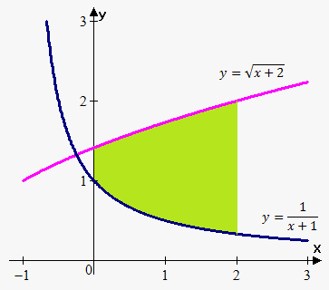 Example 1. Find the area of the region bounded above by $$${y}=\sqrt{{{x}+{2}}}$$$, bounded below by $$${y}=\frac{{1}}{{{x}+{1}}}$$$, and bounded on the sides by $$${x}={0}$$$ and $$${x}={2}$$$.
The upper boundary curve is $$${f{{\left({x}\right)}}}=\sqrt{{{x}+{2}}}$$$ and the lower boundary curve is $$${y}=\frac{{1}}{{{x}+{1}}}$$$. Therefore, $$${A}={\int_{{0}}^{{2}}}{\left(\sqrt{{{x}+{2}}}-\frac{{1}}{{{x}+{1}}}\right)}{d}{x}={\left(\frac{{2}}{{3}}{{\left({x}+{2}\right)}}^{{\frac{{3}}{{2}}}}-{\ln{{\left({x}+{1}\right)}}}\right)}{{\mid}_{{0}}^{{2}}}=$$$
$$$={\left(\frac{{2}}{{3}}\cdot{8}-{\ln{{\left({3}\right)}}}\right)}-{\left(\frac{{2}}{{3}}{{2}}^{{\frac{{3}}{{2}}}}-{\ln{{\left({1}\right)}}}\right)}=\frac{{16}}{{3}}-\frac{{4}}{{3}}\sqrt{{{8}}}-{\ln{{\left({3}\right)}}}$$$.
Now let's see how to handle situations when we are not given limits for integration.
Example 2. Find the area of the region enclosed by the parabola $$${y}={5}{x}-{{x}}^{{2}}$$$ and line $$${y}={x}$$$.
We are not given points bounds of integration here, so we need to find them.
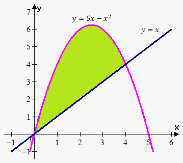
For this need to find points of intersections of curves. To do this we must solve system
$$${\left\{\begin{array}{c}{y}={5}{x}-{{x}}^{{2}}\\{y}={x}\\ \end{array}\right.}$$$.
From this $$${5}{x}-{{x}}^{{2}}={x}$$$ or $$${x}{\left({x}-{4}\right)}={0}$$$. Solutions are $$${x}={0}$$$ and $$${x}={4}$$$. Thus, points of intersection are (0,0) and (4,4)
Top boundary curve is $$${y}={5}{x}-{{x}}^{{2}}$$$ and lower boundary curve is $$${y}={x}$$$. Therefore, $$${A}={\int_{{0}}^{{4}}}{\left({\left({5}{x}-{{x}}^{{2}}\right)}-{x}\right)}{d}{x}={\int_{{0}}^{{4}}}{\left({4}{x}-{{x}}^{{2}}\right)}{d}{x}={\left({2}{{x}}^{{2}}-\frac{{1}}{{3}}{{x}}^{{3}}\right)}{{\mid}_{{0}}^{{4}}}=$$$
$$$={\left({2}\cdot{{4}}^{{2}}-\frac{{1}}{{3}}\cdot{{4}}^{{3}}\right)}={32}-\frac{{64}}{{3}}=\frac{{32}}{{3}}$$$.
Now, let's see in what situations we need to split interval of integration into parts.
Example 3. Find the area of the region enclosed by $$${y}={5}{x}-{{x}}^{{2}}$$$ and $$${y}={x}$$$ on interval $$${\left[-{1},{5}\right]}$$$.
This example is extension of example 2. We encounter here problem. Function $$${f{{\left({x}\right)}}}={5}{x}-{{x}}^{{2}}$$$ is not greater than $$${g{{\left({x}\right)}}}={x}$$$ on interval $$${\left[-{1},{5}\right]}$$$.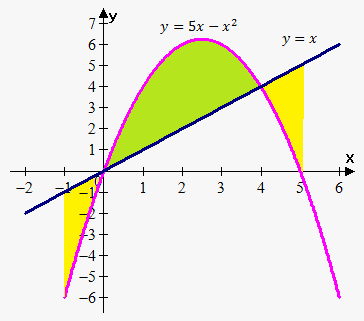
To solve this problem we must divide interval $$${\left[-{1},{5}\right]}$$$ on subintervals where $$${f{{\left({x}\right)}}}\ge{g{{\left({x}\right)}}}$$$ and where $$${g{{\left({x}\right)}}}\ge{f{{\left({x}\right)}}}$$$.
First subinterval is $$${\left[-{1},{0}\right]}$$$: here $$${f{{\left({x}\right)}}}\le{g{{\left({x}\right)}}}$$$ so $$${A}_{{1}}={\int_{{-{1}}}^{{0}}}{\left({x}-{\left({5}{x}-{{x}}^{{2}}\right)}\right)}{d}{x}=$$$
$$$={\int_{{-{1}}}^{{0}}}{\left({{x}}^{{2}}-{4}{x}\right)}{d}{x}={\left(\frac{{1}}{{3}}{{x}}^{{3}}-{2}{{x}}^{{2}}\right)}{{\mid}_{{-{1}}}^{{0}}}=-{\left(-\frac{{1}}{{3}}-{2}\right)}=\frac{{7}}{{3}}$$$.
Second subinterval is $$${\left[{0},{4}\right]}$$$: here $$${f{{\left({x}\right)}}}\ge{g{{\left({x}\right)}}}$$$ and we found area of this region in example 2, so $$${A}_{{2}}=\frac{{32}}{{3}}$$$.
Third subinterval is $$${\left[{4},{5}\right]}$$$: here again $$${f{{\left({x}\right)}}}\ge{g{{\left({x}\right)}}}$$$ so $$${A}_{{1}}={\int_{{4}}^{{5}}}{\left({x}-{\left({5}{x}-{{x}}^{{2}}\right)}\right)}{d}{x}={\int_{{4}}^{{5}}}{\left({{x}}^{{2}}-{4}{x}\right)}{d}{x}={\left(\frac{{1}}{{3}}{{x}}^{{3}}-{2}{{x}}^{{2}}\right)}{{\mid}_{{4}}^{{5}}}=$$$
$$$={\left(\frac{{1}}{{3}}\cdot{{5}}^{{3}}-{2}\cdot{{5}}^{{2}}\right)}-{\left(\frac{{1}}{{3}}\cdot{{4}}^{{3}}-{2}\cdot{{4}}^{{2}}\right)}=\frac{{7}}{{3}}$$$.
Finally total area is $$${A}=\frac{{7}}{{3}}+\frac{{32}}{{3}}+\frac{{7}}{{3}}=\frac{{46}}{{3}}$$$.
Following example shows that sometimes it is better to treat function as function of $$${y}$$$ rather than $$${x}$$$.
Example 4. Find the area enclosed by the line $$${y}={x}+{1}$$$ and parabola $$${{y}}^{{2}}={2}{x}+{5}$$$.
Here the first problem is that on different intervals we have different lower bounds. The other problem that we need express $$${y}$$$ from $$${{y}}^{{2}}={2}{x}+{6}$$$. We obtain 2 curves: $$${y}=\pm\sqrt{{{2}{x}+{5}}}$$$. This adds work to find area.
So, it is better to use formula when $$${x}$$$ is a function of $$${y}$$$.
But for educational purposes let's do it in two ways.
First find points of intersection:
$$${\left\{\begin{array}{c}{y}={x}+{1}\\{{y}}^{{2}}={2}{x}+{5}\\ \end{array}\right.}$$$
Or $$${{\left({x}+{1}\right)}}^{{2}}={2}{x}+{5}$$$. From this we have that $$${{x}}^{{2}}={4}$$$. Solving this equation we obtain that $$${x}=\pm{2}$$$.
Thus, points of intersection are (-2,-1) and (2,3).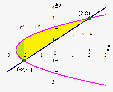
Also, point where $$${y}={0}$$$ for curve $$${{y}}^{{2}}={2}{x}+{5}$$$ is $$${x}=-\frac{{5}}{{2}}$$$.
Let's first solve regarding $$${y}$$$ as a function of $$${x}$$$. This will show the two problems we talked about.
First problem is that $$${{y}}^{{2}}={2}{x}+{5}$$$ or $$${y}=\pm\sqrt{{{2}{x}+{5}}}$$$. This gives two curves.
Second problem is that we can't integrate directly. We must divide required area into two areas: green area and yellow area, because there are different lower boundary curves:
For green area lower boundary curve is $$$-\sqrt{{{2}{x}+{5}}}$$$, so $$${A}_{{1}}={\int_{{-\frac{{5}}{{2}}}}^{{-{2}}}}{\left(\sqrt{{{2}{x}+{5}}}-{\left(-\sqrt{{{2}{x}+{5}}}\right)}\right)}{d}{x}={2}{\int_{{-\frac{{5}}{{2}}}}^{{-{2}}}}\sqrt{{{2}{x}+{5}}}{d}{x}=\frac{{2}}{{3}}{{\left({2}{x}+{5}\right)}}^{{\frac{{3}}{{2}}}}{{\mid}_{{-\frac{{5}}{{2}}}}^{{-{2}}}}=$$$
$$$=\frac{{2}}{{3}}\cdot{1}=\frac{{2}}{{3}}$$$.
For yellow area lower boundary curve is $$${y}={x}+{1}$$$, so $$${A}_{{2}}={\int_{{-{2}}}^{{{2}}}}{\left(\sqrt{{{2}{x}+{5}}}-{\left({x}+{1}\right)}\right)}{d}{x}={\int_{{-{2}}}^{{2}}}{\left(\sqrt{{{2}{x}+{5}}}-{x}-{1}\right)}{d}{x}={\left(\frac{{1}}{{3}}{{\left({2}{x}+{5}\right)}}^{{\frac{{3}}{{2}}}}-\frac{{1}}{{2}}{{x}}^{{2}}-{x}\right)}{{\mid}_{{-{2}}}^{{2}}}=$$$
$$$={9}-{2}-{2}-{\left(\frac{{1}}{{3}}-{2}+{2}\right)}=\frac{{14}}{{3}}$$$.
Therefore, $$${A}={A}_{{1}}+{A}_{{2}}=\frac{{2}}{{3}}+\frac{{14}}{{3}}=\frac{{16}}{{3}}$$$.
If we now treat $$${x}$$$ as function of $$${y}$$$ then equations of curves are: $$${x}={y}-{1}$$$ and $$${x}=\frac{{1}}{{2}}{\left({{y}}^{{2}}-{5}\right)}$$$, bounds for $$${y}$$$ are from $$$-1$$$ to $$$3$$$, so $$${A}={\int_{{-{1}}}^{{3}}}{\left({y}-{1}-\frac{{1}}{{2}}{\left({{y}}^{{2}}-{5}\right)}\right)}{d}{y}={\left(\frac{{1}}{{2}}{{y}}^{{2}}-\frac{{1}}{{6}}{{y}}^{{3}}+\frac{{3}}{{2}}{y}\right)}{{\mid}_{{-{1}}}^{{3}}}=\frac{{9}}{{2}}-\frac{{9}}{{2}}+\frac{{9}}{{2}}-{\left(\frac{{1}}{{2}}+\frac{{1}}{{6}}-\frac{{3}}{{2}}\right)}=\frac{{16}}{{3}}$$$.
As can be seen second method is much easier.
