Representing a Function
There are three possible ways to represent a function:
- analytically (by formula);
- numerically (by table of values);
- visually (by graph).
Analytical representation of a function.
This is the most common way to represent a function. We define a formula that contains arithmetic operations on constant values and the variable $$${x}$$$ that we need to perform to obtain the value of $$${y}$$$.
For example, $$${y}=\frac{{1}}{{{1}+{{x}}^{{2}}}}$$$, $$${y}={3}{{x}}^{{2}}-{5}$$$, etc.
Now, from the function $$${y}=\frac{{1}}{{{1}+{{x}}^{{2}}}}$$$, we can find that $$${y}{\left({2}\right)}=\frac{{1}}{{{1}+{{2}}^{{2}}}}=\frac{{1}}{{5}}$$$.
However, this is not the only way to represent a function. We can represent it analytically without a formula.
For example, consider the function $$${y}={\left[{x}\right]}$$$ (floor function). Clearly, $$${\left[{1}\right]}={1}$$$, $$${\left[{2.5}\right]}={2}$$$, $$${\left[\sqrt{{{13}}}\right]}={3}$$$, $$${\left[-\pi\right]}=-{4}$$$, etc., but there is no formula that expresses $$${\left[{x}\right]}$$$.
Another example is $$${f{{\left({x}\right)}}}={x}!={1}\cdot{2}\cdot{3}\cdot\ldots\cdot{x}$$$. The domain of this function is a set of natural numbers, because $$${x}$$$ can take only natural values. So, $$${f{{\left({3}\right)}}}={3}!={6}$$$, but again, there is no formula that expresses $$${x}!$$$.
Now, let's talk about the domain of the function.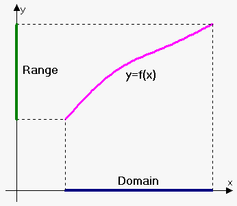
We can state the domain of the function explicitly, for example, $$${f{{\left({x}\right)}}}={{x}}^{{2}},{3}\le{x}\le{5}$$$. This means that $$${x}$$$ can change only in the interval $$${\left[{3},{5}\right]}$$$.
But often, the domain is given implicitly, i.e. the domain is all values of $$${x}$$$ where $$${f{{\left({x}\right)}}}$$$ is defined.
For example, for the function $$${f{{\left({x}\right)}}}={{x}}^{{2}}+{1}$$$, the domain is a set of all real numbers, i.e. the interval $$${\left(-\infty,\infty\right)}$$$, because the function is defined for any value of $$${x}$$$.
The domain of the function $$${h}{\left({x}\right)}=\frac{{1}}{{{x}-{2}}}$$$ is all real numbers except $$${x}={2}$$$, i.e. $$${\left(-\infty,{2}\right)}\cup{\left({2},\infty\right)}$$$. $$${x}={2}$$$ is not in the domain, because $$${h}{\left({2}\right)}$$$ is not defined (the denominator equals $$${0}$$$).
The domain of the function $$${y}{\left({x}\right)}=\sqrt{{{1}-{{x}}^{{2}}}}$$$ is $$${\left[-{1},{1}\right]}$$$, because for these values the expression under the root is non-negative, and, thus, the function $$${y}{\left({x}\right)}$$$ is defined.
Moreover, in a real-world application, we also need to make sure that the function makes sense. For example, consider the law of free fall $$${s}=\frac{{1}}{{2}}{{g{{t}}}}^{{2}}$$$. This function is defined for all $$${t}$$$ but it doesn't make sense when $$${t}<{0}$$$ (time can't be negative). Therefore, the domain of the function in the given situation is $$${\left({0},\infty\right)}$$$.
Example 1. Suppose that the perimeter of a rectangle is 24 cm. Find its area as the function of one side. Find the domain of this function.
Let's suppose that one side is $$${x}$$$ and the second side is $$${u}$$$. Then, $$${2}{x}+{2}{u}={24}$$$, or $$${u}={12}-{x}$$$.
Therefore, the area is $$${A}={x}{u}={x}{\left({12}-{x}\right)}$$$. Thus, $$${A}{\left({x}\right)}={x}{\left({12}-{x}\right)}$$$.
Since length should be positive, $$${x}>{0}$$$. Also, area should be positive; so, $$${12}-{x}>{0}$$$, or $$${x}<{12}$$$. Thus, the domain is the interval $$${\left({0},{12}\right)}$$$.
Let's work another quick example.
Example 2. State the domain of $$${f{{\left({x}\right)}}}=\frac{{1}}{{{{x}}^{{2}}-{3}{x}}}$$$.
Since $$${{x}}^{{2}}-{3}{x}={x}{\left({x}-{3}\right)}$$$ and the denominator can't equal $$${0}$$$, the domain of the function is all real numbers except $$${x}={0}$$$ and $$${x}={3}$$$.
One more quick example for practice.
Example 3. Find the domain of the function $$${f{{\left({t}\right)}}}=\sqrt{{{t}}}+{\sqrt[{{3}}]{{{t}}}}$$$.
Since the square root should be non-negative, the domain of the function is $$${t}\ge{0}$$$.
And let's do another short example before passing on.
Example 4. Find $$${f{{\left({x}+{h}\right)}}}$$$, if $$${f{{\left({x}\right)}}}=\frac{\sqrt{{{x}}}}{{{{x}}^{{2}}+{3}{x}+{4}}}$$$.
$$${f{{\left({x}+{h}\right)}}}=\frac{\sqrt{{{x}+{h}}}}{{{{\left({x}+{h}\right)}}^{{2}}+{3}{\left({x}+{h}\right)}+{4}}}$$$.
Numerical (tabular) representation of a function.
In real life, the dependence between variables is formed based on experiments or observations. For example, at any given time $$${t}$$$, we can calculate the world population $$${N}$$$. We say that $$${N}$$$ is a function of $$${t}$$$ but can't find an explicit formula to express this. All we have is a table of values as below:
| $$${t}$$$ (in years) | 1970 | 1980 | 1990 | 2000 | 2010 |
| $$${N}$$$ (in millions of people) | 3835 | 4100 | 4545 | 5600 | 7300 |
However, in further topics of calculus, we will be able to find a function that will approximate these values.
Graphical representation of a function.
Although in calculus functions are not defined graphically, graphical representation is very helpful in studying functions.
Suppose that we are given a function $$${y}={f{{\left({x}\right)}}}$$$ with the domain $$${X}$$$. Imagine a plane with two 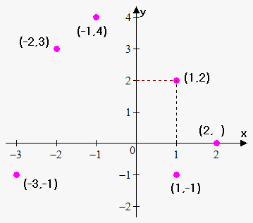 perpendicular axes: the x-axis and the y-axis. Consider a pair of corresponding values $$${x}$$$ and $$${y}$$$, where $$${x}$$$ is taken from set $$${X}$$$ and $$${y}={f{{\left({x}\right)}}}$$$. The image of this pair is the point $$${A}{\left({x},{y}\right)}$$$ with the x-coordinate $$${x}$$$ and the y-coordinate $$${y}$$$. When the variable $$${x}$$$ is changing within the interval $$${X}$$$, this point describes some curve. This curve is the graph of the function $$${y}={f{{\left({x}\right)}}}$$$.
So, to draw the graph of the function, take from the interval $$${X}$$$ points that are close to each other: $$${x}_{{1}},{x}_{{2}},{x}_{{3}},\ldots{x}_{{n}}$$$. Now, find the corresponding y-values: $$${y}_{{1}}={f{{\left({x}_{{1}}\right)}}}$$$, $$${y}_{{2}}={f{{\left({x}_{{2}}\right)}}}$$$,..., $$${y}_{{n}}={f{{\left({x}_{{n}}\right)}}}$$$.
Draw the points $$${\left({x}_{{1}},{y}_{{1}}\right)}$$$, $$${\left({x}_{{2}},{y}_{{2}}\right)}$$$,..., $$${\left({x}_{{n}},{y}_{{n}}\right)}$$$. Connect these points by a smooth curve. We've obtained the graph of the function. Note: the more points you take, the more accurate graph you will obtain.
Let's move on to practical examples.
Example 5. Draw the graph of the function $$${y}={{x}}^{{2}}$$$ on the interval $$${\left[{0},{1}\right]}$$$.
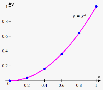 Let's take the following points: $$${x}_{{1}}={0}$$$, $$${x}_{{2}}={0.2}$$$, $$${x}_{{3}}={0.4}$$$, $$${x}_{{4}}={0.6}$$$, $$${x}_{{5}}={0.8}$$$, $$${x}_{{6}}={1}$$$.
Now, find the corresponding y-values: $$${y}_{{1}}={{\left({0}\right)}}^{{2}}={0}$$$, $$${y}_{{2}}={{\left({0.2}\right)}}^{{2}}={0.04}$$$, $$${y}_{{3}}={{\left({0.4}\right)}}^{{2}}={0.16}$$$, $$${y}_{{4}}={{\left({0.6}\right)}}^{{2}}={0.36}$$$, $$${y}_{{5}}={{\left({0.8}\right)}}^{{2}}={0.64}$$$, $$${y}_{{6}}={{\left({1}\right)}}^{{2}}={1}$$$.
Draw the points $$${\left({0},{0}\right)}$$$, $$${\left({0.2},{0.04}\right)}$$$, $$${\left({0.4},{0.16}\right)}$$$, $$${\left({0.6},{0.36}\right)}$$$, $$${\left({0.8},{0.64}\right)}$$$, $$${\left({1},{1}\right)}$$$ on the xy-plane and connect them by a smooth curve.
And a bit more work to memorize it better.
Example 6. Consider the function whose graph is shown to the left. Find $$${f{{\left({0}\right)}}}$$$, $$${f{{\left({2}\right)}}}$$$ and state the domain and the range of $$${f{}}$$$.
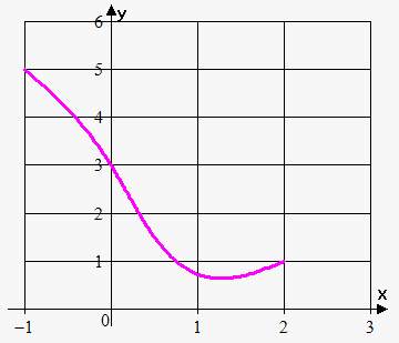 We take the point $$${x}={0}$$$ and move up until the intersection of the curve. The intersection is at the point $$${3}$$$; so, $$${f{{\left({0}\right)}}}={3}$$$. Similarly, $$${f{{\left({2}\right)}}}={1}$$$.
The function is defined when $$$-{1}\le{x}\le{3}$$$; therefore, the domain of the function is the interval $$${\left[-{1},{3}\right]}$$$, and the range is $$${\left[{1},{5.5}\right]}$$$.
The graph of the function is a curve in the xy-plane. But the question arises: which curves in the xy-plane are graphs of functions? This is answered by the following test.
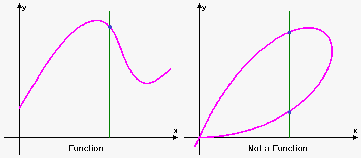
Vertical line test. A curve in the xy-plane is the graph of a function of $$${x}$$$ if and only if no vertical line intersects the curve more than once.
Graphical representation allows us to determine easily whether the curve is a function.
Consider the graph of the function $$${{y}}^{{2}}+{{x}}^{{2}}={4}$$$. It is a cirlcle with a radius of 2. Clearly, it is not a function.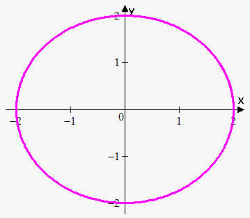
To see why it is so, express $$${y}$$$ in terms of $$${x}$$$: $$${{y}}^{{2}}={4}-{{x}}^{{2}}$$$, or $$${y}=\pm\sqrt{{{4}-{{x}}^{{2}}}}$$$. Because of $$$\pm$$$, we have two values of $$${y}$$$ for every value of $$${x}$$$. Also, as can be seen from the graph, the function fails the vertical line test.
Parametric representation of a function.
Parametric representation is a slightly changed form of representing a function by a formula.
When we define a function by a formula, we use the following record: $$${y}={f{{\left({x}\right)}}}$$$, where $$${f{}}$$$ is some formula.
But often, it is more convenient to represent a function using two functions and a parameter.
If we define a function as $$${x}={u}{\left({t}\right)},{y}={v}{\left({t}\right)}$$$, by changing the value of $$${t}$$$ (parameter), we can find the corresponding pairs of $$${x}$$$ and $$${y}$$$.
In general, we set some restrictions on $$${t}$$$. If we require $$${a}\le{t}\le{b}$$$, the point $$${\left({u}{\left({a}\right)},{v}{\left({a}\right)}\right)}$$$ is called initial, and the point $$${\left({u}{\left({b}\right)},{v}{\left({b}\right)}\right)}$$$ is called terminal.
In some cases (but not always), it is possible to eliminate the paremeter $$${t}$$$ and obtain the standard representation of $$${y}$$$ as a function of $$${x}$$$ (or $$${x}$$$ as a function of $$${y}$$$).
Also, note that parametric equations can generate curves that are not functions.
Example 7. Draw the graph of the function $$${x}={{t}}^{{3}}+{1},{y}={{t}}^{{2}}-{1}$$$, $$$-{2}\le{t}\le{2}$$$.
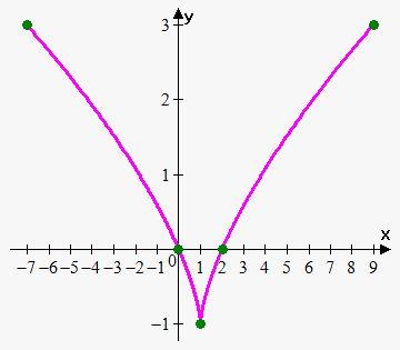 Let's find a couple of points that correspond to different values of $$${t}$$$.
| $$${t}$$$ | $$${x}$$$ | $$${y}$$$ |
| $$$-{2}$$$ | $$${{\left(-{2}\right)}}^{{3}}+{1}=-{7}$$$ | $$${{\left(-{2}\right)}}^{{2}}-{1}={3}$$$ |
| $$$-{1}$$$ | $$${{\left(-{1}\right)}}^{{3}}+{1}={0}$$$ | $$${{\left(-{1}\right)}}^{{2}}-{1}={0}$$$ |
| $$${0}$$$ | $$${{0}}^{{3}}+{1}={1}$$$ | $$${{0}}^{{2}}-{1}=-{1}$$$ |
| $$${1}$$$ | $$${{1}}^{{3}}+{1}={2}$$$ | $$${{1}}^{{2}}-{1}={0}$$$ |
| $$${2}$$$ | $$${{2}}^{{3}}+{1}={9}$$$ | $$${{2}}^{{2}}-{1}={3}$$$ |
The graph of this function is shown to the right.
Note that in this case we can eliminate the parameter $$${t}$$$: from the first equation, $$${t}={{\left({x}-{1}\right)}}^{{\frac{{1}}{{3}}}}$$$; plugging this equation for $$${t}$$$ into the second equation gives $$${y}={{\left({x}-{1}\right)}}^{{\frac{{2}}{{3}}}}-{1}$$$.
And one more final example.
Example 8. Draw the function $$${x}={{t}}^{{2}}+{t},{y}={{t}}^{{3}}-{{t}}^{{2}}$$$, $$$-{2}\le{t}\le{2}$$$.
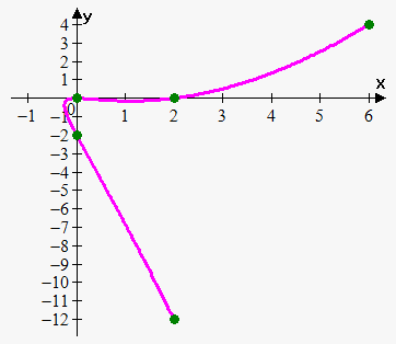 Let's find a couple of points that correspond to different values of $$${t}$$$.
| $$${t}$$$ | $$${x}$$$ | $$${y}$$$ |
| $$$-{2}$$$ | $$${{\left(-{2}\right)}}^{{2}}+{\left(-{2}\right)}={2}$$$ | $$${{\left(-{2}\right)}}^{{3}}-{{\left(-{2}\right)}}^{{2}}=-{12}$$$ |
| $$$-{1}$$$ | $$${{\left(-{1}\right)}}^{{2}}+{\left(-{1}\right)}={0}$$$ | $$${{\left(-{1}\right)}}^{{3}}-{{\left(-{1}\right)}}^{{2}}=-{2}$$$ |
| $$${0}$$$ | $$${{0}}^{{2}}+{0}={0}$$$ | $$${{0}}^{{3}}-{{0}}^{{2}}={0}$$$ |
| $$${1}$$$ | $$${{1}}^{{2}}+{1}={2}$$$ | $$${{1}}^{{3}}-{{1}}^{{2}}={0}$$$ |
| $$${2}$$$ | $$${{2}}^{{2}}+{2}={6}$$$ | $$${{2}}^{{3}}-{{2}}^{{2}}={4}$$$ |
Note that this is not a function, because it fails the vertical line test. Also, it is very hard to eliminate the parameter $$${t}$$$.
